Differential Equation Visualization - Dampened Pendulum System

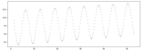
Experimenting with using basic Python to visualize a simple differential equation - a simple harmonic motion pendulum with some air resistance using different initial conditions:

$$ d^2θ/dt^2 = - μ * (dθ/dt) - (g/L) * sin(θ) $$

Code (Available on Github)

import numpy as np
from matplotlib import pyplot as plt

g=9.8  # Gravity
L=1  # Pendulum Length
mu = 0.1  # Friction Coefficient
n = 10000  # Number of dt Time Steps
t = np.pi / 3  # Initial Condition (Theta / "position")
td = 1  # Initial Condition (dTheta / "velocity")
dt = 0.02  # Time Differential

# set up figure
fig = plt.figure()
ax = fig.add_subplot()


for i in range(n):  # For each dt increment
    tdd = -mu * td - (g/L) * np.sin(t)  # Calculate d2Theta (second derivative)
    td = td + tdd*dt  # Approximate dTheta using d2Theta
    t = t + td*dt  # Approximate theta using dTheta

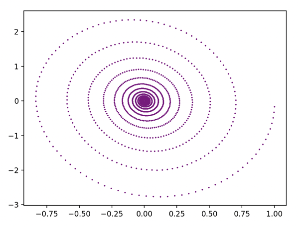
    # Plot Theta "Position" (X-axis) vs. dTheta "Velocity" (Y-Axis)
    ax.plot(t,td,marker="o", markersize=1, markeredgecolor="purple", markerfacecolor="green")
    plt.pause(0.001)

Examples (Different Initial Conditions)

High Friction - Low dθ/dt

μ = 0.5, dθ/dt = 1

High Friction - High dθ/dt

μ = 0.5, dθ/dt = 10

Low Friction - High dθ/dt

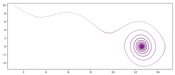
μ = 0.1, dθ/dt = 10